FFT (Fast Fourier Transform) 笔记
问题
函数 $f(t)$ 的 Fourier Transform 为
$$ \begin{align*} \mathcal{F}(\omega) = \int_{-\infty} ^{\infty} f(t) e^{-\mathrm{i} \omega t} \mathrm{d}t \end{align*} $$假函数 $f(t)$ 它只在 $t \in (0, T)$ 之间有取值, 那么上式就变为
$$ \begin{align*} \mathcal{F}(\omega) = \int_{0} ^{T} f(t) e^{-\mathrm{i} \omega t} \mathrm{d}t \end{align*} $$如此做 Fourier Transform , 需要算积分.
DFT (Discrete Fourier Transform)
如果用计算机进行数值上的计算, 会对积分进行离散化, 那么就变成了离散的 Fourier Transform .
假设将积分均匀地分成
如果
精髓
进行数值计算时, 对应每一个 $\omega$ 都要算一个求和. 我们只能进行有限次数的计算, 因此必须要选取特定的 $\omega$ 进行计算, 也就是 同样要对 $\omega$ 进行离散化.
FFT 将 $\omega$ 同样离散化成
我觉得接下来是 FFT 最关键的一步. 这也是我之前对于 FFT 不明白的地方.
首先假设 $\omega$ 的间距是 $\Delta \omega$ . 那么原式就变为
$$ \begin{align*} F(m \Delta\omega) = \frac{T}{N} \sum_{n=0}^{N-1} f\left( \frac{T}{N}n \right) e^{-\mathrm{i}2\pi \frac{1}{2\pi} m\Delta\omega \frac{T}{N}n} \end{align*} $$其中 $m = 0, 1, 2, \cdots N-1$ . FFT 让
$$ \begin{align*} \frac{1}{2\pi} \Delta \omega T =1 \end{align*} $$这样的话, $\Delta \omega$ 就选定了
$$ \begin{align*} \Delta \omega = \frac{2\pi}{T} \end{align*} $$结论
这样选取 $\Delta\omega$ 的结果就使原式变成了
$$ \begin{align*} F(m \Delta\omega) = \frac{T}{N} \sum_{n=0}^{N-1} f\left( \frac{T}{N}n \right) e^{-\mathrm{i}\frac{2\pi}{N} m n} \end{align*} $$这实际上就变成了一个矩阵运算
$$ \begin{align*} \left( \begin{array}{c} F (0)\\ F (\Delta\omega)\\ F (2\Delta\omega)\\ F (3\Delta\omega)\\ \vdots \\ F ((N-1)\Delta\omega)\\ \end{array} \right) = \frac{T}{N} \left( \begin{array}{cccccc} 1 & 1 & 1 & 1 & \cdots & 1 \\ 1 & e^{-\mathrm{i}\frac{2\pi}{N}} & e^{-\mathrm{i}\frac{2\pi}{N}\cdot 2} & e^{-\mathrm{i}\frac{2\pi}{N}\cdot 3} & \cdots & e^{-\mathrm{i}\frac{2\pi}{N}\cdot(N-1)} \\ 1 & e^{-\mathrm{i}\frac{2\pi}{N}\cdot 2} & e^{-\mathrm{i}\frac{2\pi}{N}\cdot 2\times 2} & e^{-\mathrm{i}\frac{2\pi}{N}\cdot 2\times 3} & \cdots & e^{-\mathrm{i}\frac{2\pi}{N}\cdot 2\times(N-1)} \\ 1 & e^{-\mathrm{i}\frac{2\pi}{N}\cdot 3} & e^{-\mathrm{i}\frac{2\pi}{N}\cdot 3\times 2} & e^{-\mathrm{i}\frac{2\pi}{N}\cdot 3\times 3} & \cdots & e^{-\mathrm{i}\frac{2\pi}{N}\cdot 3\times(N-1)} \\ \vdots & \vdots & \vdots & \vdots & \ddots & \vdots \\ 1 & e^{\mathrm{-i}\frac{2\pi}{N}\cdot (N-1)} & e^{-\mathrm{i}\frac{2\pi}{N}\cdot (N-1)\times 2} & e^{-\mathrm{i}\frac{2\pi}{N}\cdot (N-1)\times 3} & \cdots & e^{-\mathrm{i}\frac{2\pi}{N}\cdot (N-1)\times(N-1)} \\ \end{array} \right) \left( \begin{array}{c} f (0)\\ f \left( \frac{T}{N} \right)\\ f \left( 2\frac{T}{N} \right)\\ f \left( 3\frac{T}{N} \right)\\ \vdots \\ f \left( (N-1)\frac{T}{N} \right)\\ \end{array} \right) \end{align*} $$可以发现, 对于给定
简的可以手算的例子
我之所以会对这个感兴趣, 是因为我想要用电脑对一些函数做 Fourier Transform ,于是得知有 FFT 这样现成的程序. 但是 FFT 给出的结果 却令我难过. 因为我不知道它给出的是些什么. 一堆复数, 画出来形状也很奇怪. 不知道输出的结果对应的横坐标.
既然这样, 只要知道了 FFT 的原理, 就一定能够得出我想要的答案. 答案就是它的输出, 是上式等号左边那一个列向量的数值然后把 $\frac{T}{N}$ 除掉, 也就是 $F(m\Delta\omega)\frac{N}{T}$
参考书上的例子, 拿一个 $N = 4$ 的例子, 进行手算, 然后与程序给出的结果对比, 便能够验证上面的猜想
$N = 4$ 的例子: 假设函数 $f(t)$ 离散化之后的四个数值为 $\{1, 1, 0, 0\}$ , 也就是说
$$ \begin{align*} f\left(\frac{0T}{4}\right) = 1 \\ f\left(\frac{T}{4}\right) = 1\\ f\left(\frac{2T}{4}\right) = 0\\ f\left(\frac{3T}{4}\right) = 0 \end{align*} $$那么
$$ \begin{align*} \frac{4}{T}F(0\cdot\Delta\omega) &= 1\cdot f\left(\frac{0T}{4}\right) + 1\cdot f\left(\frac{T}{4}\right) + 1\cdot f\left(\frac{2T}{4}\right) + 1\cdot f\left(\frac{3T}{4}\right) \\ &= 1\cdot 1 + 1\cdot 1 +1 \cdot 0 + 1\cdot 0\\ &= 2\\ \frac{4}{T}F(1\cdot\Delta\omega) &= 1\cdot f\left(\frac{0T}{4}\right) + e^{-\mathrm{i}\frac{2\pi}{4}}\cdot f\left(\frac{T}{4}\right) + e^{-\mathrm{i}\frac{2\pi}{4}\cdot 2}\cdot f\left(\frac{2T}{4}\right) + e^{-\mathrm{i}\frac{2\pi}{4}\cdot 3}\cdot f\left(\frac{3T}{4}\right) \\ & = 1\cdot 1 + (-\mathrm{i})\cdot 1 +(-1) \cdot 0 + (\mathrm{i})\cdot 0\\ &= 1 - \mathrm{i}\\ \frac{4}{T}F(2\cdot\Delta\omega) &= 1\cdot f\left(\frac{0T}{4}\right) + e^{-\mathrm{i}\frac{2\pi}{4}\cdot 2}\cdot f\left(\frac{T}{4}\right) + e^{-\mathrm{i}\frac{2\pi}{4}\cdot 2\times 2}\cdot f\left(\frac{2T}{4}\right) + e^{-\mathrm{i}\frac{2\pi}{4}\cdot 2\times 3}\cdot f\left(\frac{3T}{4}\right) \\ & = 1\cdot 1 + (-1)\cdot 1 +1 \cdot 0 + (-1)\cdot 0\\ &= 0\\ \frac{4}{T}F(3\cdot\Delta\omega) &= 1\cdot f\left(\frac{0T}{4}\right) + e^{-\mathrm{i}\frac{2\pi}{4}\cdot 3}\cdot f\left(\frac{T}{4}\right) + e^{-\mathrm{i}\frac{2\pi}{4}\cdot 3\times 2}\cdot f\left(\frac{2T}{4}\right) + e^{-\mathrm{i}\frac{2\pi}{4}\cdot 3\times 3}\cdot f\left(\frac{3T}{4}\right)\\ & = 1\cdot 1 + (\mathrm{i})\cdot 1 +( - 1) \cdot 0 + (-\mathrm{i})\cdot 0\\ &= 1 + \mathrm{i} \end{align*} $$也就是
$$ \begin{align*} \left( \begin{array}{c} 2 \\ 1-i \\ 0 \\ 1+i \end{array} \right) = \left( \begin{array}{cccc} 1&1&1&1 \\ 1&-\mathrm{i}&-1&\mathrm{i}\\ 1&-1&1&-1 \\ 1&\mathrm{i}&-1&-\mathrm{i} \end{array} \right) \left( \begin{array}{c} 1 \\ 1 \\ 0 \\ 0 \end{array} \right)\end{align*} $$然后用 Numpy 中的 numpy.fft.fft() 函数计算
import numpy as np
f = ([1,1,0,0])
F = np.fft.fft(f)
print(F)
输出结果为
[2.+0.j 1.-1.j 0.+0.j 1.+1.j]
验证了前面对于 FFT 的原理理解.
输出结果分析
输出的对称性
变换矩阵中的元素
$$ \begin{align*} e^{-\mathrm{i}\frac{2\pi}{N}mn} \end{align*} $$当
也就是说同一列中,
很明显, 手算的例子符合这一结论.
三角函数和 e 指数形式的 Fourier Transform 之间的联系
对于满足周期为
其中 $\omega=\frac{2\pi}{T}$ . 由于三角函数正交且归一到半个周期上, 所以展开系数为
$$ \begin{align*} a_n = \frac{2}{T} \int_{0}^{T} f(t)\cos (n\omega t) \mathrm{d} t \\ b_n = \frac{2}{T} \int_{0}^{T} f(t)\sin (n\omega t) \mathrm{d} t \end{align*} $$如果把三角函数用
最后一个等号利用了 $a_n = a_{-n}, b_n = -b_{-n}, b_0 = 0$ . 而
$$ \begin{align*} \frac{a_n -\mathrm{i}b_n}{2} =& \frac{2}{T} \int_{0}^{T} f(t)\frac{\cos (n\omega t) - \mathrm{i}\sin(n\omega t)}{2} \mathrm{d} t \\ =& \frac{1}{T} \int_{0}^{T} f(t)e^{-\mathrm{i}n\omega t} \mathrm{d} t \end{align*} $$若令
$$ \begin{align*} \frac{a_n - \mathrm{i}b_n}{2}T = \mathcal{F}_n \end{align*} $$则有
$$ \begin{align*} \mathcal{F}_n = & \int_{0} ^{T} f(t) e^{-\mathrm{i} n \omega t} \mathrm{d}t \\ f(t) = & \frac{1}{T} \sum_{n=-\infty}^{\infty} \mathcal{F}_n e^{\mathrm{i}n\omega t} \end{align*} $$这也和之前 Fourier Transform 总结中的一致.
输出结果中有价值的部分
输出结果的实部和虚部对应同一频率的振幅, 只不过实部是正弦部分, 虚部是余弦部分. 所以用其模长来刻画 Fourier Transform 的结果.
而且输出的结果具有对称性, 所以只取前 $\frac{N}{2}+1$ 个结果即可得到变换的全部信息.
Python 程序示例
三角函数的例子
用 Numpy 中的 numpy.fft.fft() 函数计算三角函数
的 Fourier Transform
import numpy as np
import matplotlib.pyplot as plt
N = 1024  #离散化成N个点
T =8*np.pi #输入T的值
t = np.linspace(0,T,N) #离散化t
f = np.sin(17*t) + 3*np.sin(57*t) + 2*np.sin(97*t) #f(t)的表达式
F = np.fft.fft(f) #进行FFT
tf = np.linspace(0,N*np.pi/T,N//2 + 1) #设置 \omega 坐标轴,
plt.plot(tf, np.abs(F[:N//2+1])) #以 \omega 为横轴, 以 F 为纵轴画图. 由于对称性只取前(N/2+1 个点)
plt.xlabel("$\omega$")
plt.ylabel("$F(\omega)$")
plt.title("The Results of FFT")
plt.show()
结果
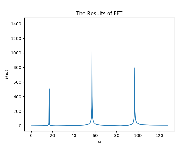
正如预期, 分别在频率为 $17, 57, 97$ 出现峰. $57$ 的峰最高, $97$ 次之, $17$ 最低.
高斯函数的例子
用 Numpy 中的 numpy.fft.fft() 函数高斯函数
和
$$ \begin{align*} f_2(t) = e^{-10t^{2}} \end{align*} $$的 Fourier Transform
import numpy as np
import matplotlib.pyplot as plt
N = 512  #离散化成N个点
T =30 #输入T的值
t = np.linspace(0,T,N) #离散化t
f1 = np.exp(-t**2) #f(t)的表达式
f2 = np.exp(-10*t**2)
F1 = np.fft.fft(f1) #进行FFT
F2 = np.fft.fft(f2) #进行FFT
tf = np.linspace(0,N*np.pi/T,N//2 + 1) #设置 \omega 坐标轴,

plt.subplot(211) #两行一列, 第一个图
plt.plot(tf, np.abs(F1[:N//2+1])) #以 \omega 为横轴, 以 F1 为纵轴画图. 由于对称性只取前(N/2+1 个点)
plt.ylabel("$F_1(\omega)$")
plt.subplot(212) #两行一列, 第二个图
plt.plot(tf, np.abs(F2[:N//2+1])) #
plt.xlabel("$\omega$")
plt.ylabel("$F_2(\omega)$")
plt.suptitle("The Results of FFT")
plt.show()
结果为
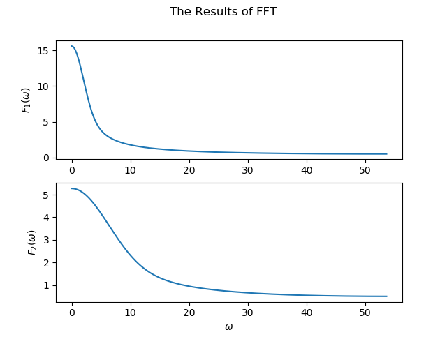
这也符合预期, 原来更尖的高斯函数, 变换之后变得更平.
致谢与参考书
-
苏变萍, 陈东立 编 复变函数与积分变换(第二版)
-
感谢 Fan Yang 师兄的讨论